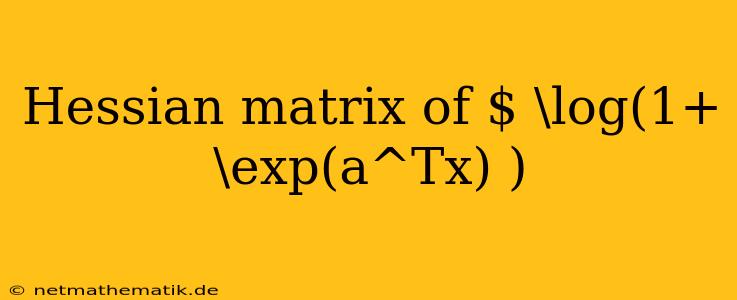
The Hessian matrix of $\log(1+\exp(a^Tx))$ is a fundamental concept in machine learning, particularly in the context of logistic regression and deep learning. This matrix, which captures the second-order partial derivatives of the function, plays a crucial role in understanding the curvature of the loss function and optimizing the model's parameters. In this article, we will delve into the detailed derivation of the Hessian matrix for this specific function, explore its properties, and highlight its significance in practical applications.
Understanding the Function and its Derivatives
The function $\log(1+\exp(a^Tx))$ is commonly used in logistic regression, where it represents the sigmoid function. This function maps any real-valued input to a value between 0 and 1, representing the probability of a binary outcome. Here, $a$ is a vector of parameters, $x$ is the input feature vector, and $a^Tx$ denotes the dot product.
Before we proceed to the Hessian matrix, let's first understand the first-order derivatives of this function.
First-order Derivatives: The Gradient
The gradient, denoted as $\nabla f(x)$, is a vector that contains all the first-order partial derivatives of the function. For our function, $f(x) = \log(1+\exp(a^Tx))$, the gradient is:
$\nabla f(x) = \frac{\exp(a^Tx)}{1+\exp(a^Tx)}a $
The gradient points in the direction of the steepest ascent of the function. In machine learning, it is used in gradient descent algorithms to iteratively update model parameters to minimize the loss function.
Deriving the Hessian Matrix
The Hessian matrix, denoted as $H(x)$, is a square matrix that contains all the second-order partial derivatives of the function. Each element $H_{ij}$ represents the partial derivative of the function with respect to $x_i$ and $x_j$:
$H_{ij}(x) = \frac{\partial^2 f(x)}{\partial x_i \partial x_j}$
To derive the Hessian matrix of $\log(1+\exp(a^Tx))$, we need to calculate all the second-order partial derivatives. This can be achieved by differentiating the gradient vector with respect to each $x_i$.
Calculating the Second-order Derivatives
Let's start by differentiating the gradient with respect to $x_i$:
$\frac{\partial}{\partial x_i} \left(\frac{\exp(a^Tx)}{1+\exp(a^Tx)}a \right) = \frac{\exp(a^Tx)(1+\exp(a^Tx))a_i - \exp(a^Tx)\exp(a^Tx)a_i}{(1+\exp(a^Tx))^2} $
Simplifying the expression, we obtain:
$\frac{\partial^2 f(x)}{\partial x_i \partial x_j} = \frac{\exp(a^Tx)}{(1+\exp(a^Tx))^2} a_i a_j$
This equation represents the $ij$-th element of the Hessian matrix.
The Hessian Matrix in Matrix Form
Using the derived expression, we can write the Hessian matrix in a compact matrix form:
$H(x) = \frac{\exp(a^Tx)}{(1+\exp(a^Tx))^2} aa^T$
This matrix is a rank-one matrix, as it is the outer product of two vectors: $a$ and $a^T$. This property is important for understanding the behavior of the Hessian matrix.
Properties and Significance of the Hessian Matrix
The Hessian matrix holds crucial information about the curvature of the function. Understanding its properties provides insights into the optimization process and the stability of the model.
Curvature and Convexity
The Hessian matrix is directly related to the curvature of the function. A positive definite Hessian matrix indicates a convex function, while a negative definite Hessian matrix indicates a concave function. For a function to have a minimum point, the Hessian matrix must be positive definite at that point. This property is fundamental in optimization, as it guarantees that a local minimum is also a global minimum.
Gradient Descent and Hessian Matrix
In gradient descent algorithms, the Hessian matrix plays a critical role. By considering the second-order information, the Hessian matrix helps to determine the optimal step size and direction of movement in the parameter space. Using the inverse of the Hessian matrix, known as the inverse Hessian or the Hessian matrix, can lead to faster convergence and more accurate solutions compared to traditional gradient descent methods.
Regularization and Hessian Matrix
In machine learning, regularization techniques are used to prevent overfitting by adding a penalty term to the loss function. The Hessian matrix can be used to understand the impact of regularization on the optimization process. For instance, L2 regularization, which adds a squared penalty on the model parameters, can be interpreted as modifying the Hessian matrix by adding a diagonal matrix to it. This modification alters the curvature of the loss function, encouraging the model to have smaller parameter values.
Conclusion
The Hessian matrix of $\log(1+\exp(a^Tx))$ is a powerful tool in machine learning, providing insights into the curvature of the loss function and impacting optimization algorithms. Understanding its properties and its role in different aspects of machine learning is crucial for building efficient and robust models. By leveraging the information encoded in the Hessian matrix, practitioners can enhance the optimization process, improve the accuracy of predictions, and gain a deeper understanding of their models. The Hessian matrix of $\log(1+\exp(a^Tx))$ remains an essential concept for researchers and practitioners in the field of machine learning, contributing significantly to the development of advanced algorithms and improved model performance.
